Open Access | Research Article
This work is licensed under a Creative
Commons Attribution-ShareAlike 4.0 International License.
KDClassifier: A urinary proteomic spectra analysis tool based on machine learning for the classification of kidney diseases
# These authors contributed equally to this work.
* Corresponding author: Hao Yang
Mailing address: West China Hospital/West China Medical
School, Sichuan University, Chengdu, 610041, China.
E-mail: yanghao@scu.edu.cn
* Corresponding author: Guisen Li
Mailing address: Sichuan Provincial People’s Hospital, University
of Electronic Science and Technology of China, Chengdu
611731, China.
E-mail: guisenli@163.com
Received: 23 July 2021 / Accepted: 6 september 2021
DOI: 10.31491/APT.2021.09.064
Abstract
Background: We aimed to establish a novel diagnostic model for kidney diseases by combining artificial
intelligence
with complete mass spectrum information from urinary proteomics.
Kidney disease classification, urinary proteomics, machine learning algorithm,
diagnosis, artificial
intelligence
Methods: We enrolled 134 patients (IgA nephropathy, membranous nephropathy, and diabetic kidney
disease)
and 68 healthy participants as controls, with a total of 610,102 mass spectra from their urinary proteomic
profiles.
The training data set (80%) was used to create a diagnostic model using XGBoost, random forest (RF), a
support vector machine (SVM), and artificial neural networks (ANNs). The diagnostic accuracy was evaluated
using a confusion matrix with a test dataset (20%). We also constructed receiver operating-characteristic,
Lorenz,
and gain curves to evaluate the diagnostic model.
Results: Compared with the RF, SVM, and ANNs, the modified XGBoost model, called Kidney Disease
Classifier
(KDClassifier), showed the best performance. The accuracy of the XGBoost diagnostic model was 96.03%. The
area under the curve of the extreme gradient boosting (XGBoost) model was 0.952 (95% confidence interval,
0.9307–0.9733). The Kolmogorov-Smirnov (KS) value of the Lorenz curve was 0.8514. The Lorenz and gain
curves showed the strong robustness of the developed model.
Conclusion:The KDClassifier achieved high accuracy and robustness and thus provides a potential
tool for the
classification of kidney diseases.
Keywords
Introduction
Chronic kidney disease (CKD) has become a major public health problem and significant burden globally owing to
its global incidence rate of >10% [1, 2]. Persisting renal
damage and loss of renal function are the main clinical
characteristics of CKD. Despite the continuous effort of
nephropathologists, the incidence, prevalence, mortality
rate, and disability-adjusted life-years of CKD remain
extremely high and have even increased significantly in
recent decades [2]. Kidney diseases are mainly evaluated
on the basis of persistent proteinuria, hematuria, and
clinical impairment of the renal function, and decreased
glomerular filtration rate (GFR) [3, 4]. However, the
clinical characteristics of kidney diseases with different
pathological categories are obviously different, including
primary glomerular diseases such as immunoglobulin A
(IgA) nephropathy (IgAN) and membranous nephropathy (MN), and secondary glomerular diseases such as diabetic
kidney disease (DKD). To improve the outcomes of CKD,
strategies to distinguish kidney diseases more easily and
early and more precise treatment methods are important.
With the innovation of puncture biopsy technology, renal
biopsies have become the most critical technology for the
pathological diagnosis and elucidation of various kidney
diseases in recent years [5-7]. Renal biopsy is the gold
standard for diagnosis, treatment, and predicting the prognosis
of kidney diseases through a pathological analysis.
A series of important advances in renal pathology have
promoted the understanding of the pathogenesis of renal
diseases. In the future, an artificial intelligence-assisted
pathological analysis tool will expand the understanding
of renal pathological lesions and the pathogenesis of kidney
disease [7-9]. However, as an
invasive procedure, kidney
biopsy may incur some ineluctable complications, of
which the most frequent is macrohematuria with or without
the need for blood transfusion [10, 11]. In addition,
many patients could not undergo renal biopsy because of
relative or absolute contraindications. Therefore, the identification
of novel noninvasive biomarkers or development
of methods to improve the diagnostic efficiency, monitoring,
and treatment of CKD is needed.
Some existing studies have shown that urine, serum metabolite,
and protein have potential clinical applications
as biomarkers [12-14].
Proteins are considered the final
products of gene-environment interactions and a physiological
steady-state. A single highly specific and unique
biomarker (e.g., an M-type phospholipase A2 receptor for
MN) is certainly the best choice [15]; however, such biomarker
is unavailable for clinically noninvasive diagnosis
of numerous kidney diseases such as IgAN or DKD. The
measurement of the levels of various urinary proteins can
be combined with the use of available clinical biochemistry
indexes, which have potential usefulness for clinical
diagnosis, patient stratification, and therapeutic monitoring
[16]. Proteomics provides new insight into biomarker
discovery and has dramatically widened our appreciation
of pathological mechanisms. New analytical tools with
high accuracy have made proteomics easier and quantifiable,
allowing the acquisition of information from biological
samples [17].
The mass spectra of urinary proteomes produced by
liquid
chromatography tandem mass spectrometry (LC-MS/MS)
are big data sets containing rich information. The existing
software cannot interpret all spectral information. With
the development of mass spectrometry and machine learning
algorithms, the extraction of spectrum features from
the urinary proteome of each disease entity by using an
advanced mass spectrometer and machine learning algorithms
can save a lot of time and lead to a more accurate
reporting of results. Therefore, we believe that the use of
all mass spectral information from a urinary proteome, as
provided through advanced mass spectrometry, can be an
effective potential research direction to improve the accuracy
of CKD diagnosis.
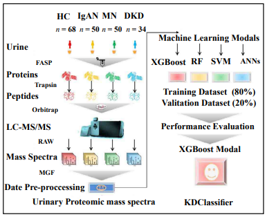
In this study, we trained and validated a diagnostic machine
learning model using more than 600,000 mass spectra
from the urinary proteomes produced using LC-MS/
MS in patients with CKD. This method permits the rapid
extraction of spectrum features from human urine (including
soluble proteins, exosomes, and other membrane
elements). We compared four machine learning models,
namely an artificial neural network (ANN), a support vector
machine (SVM), a decision tree (DT), and extreme
gradient boosting (XGBoost). We chose the most accurate
model and evaluated its performance in the classification
of patients with CKD and healthy controls (HC). Finally,
the XGBoost model, called Kidney Disease Classifier
(KDClassifier), showed the best performance in distinguishing
different patients with CKD by using the mass
spectra from the urinary proteomes of the patients with
IgAN, MN, and DKD and the HC group. The mass spectra
data on the urinary proteomics were deposited into the
ProteomeXchange Consortium through the PRIDE partner
repository using the dataset identifier PXD018996.
Materials and methods
Study population
All patients and health controls were recruited from Sichuan
Provincial People’s Hospital from September 2019 to
May 2020. Written consent was obtained from the participants
prior to the physical examination or biopsy procedure.
All the participants were recruited on a voluntary basis.
Our study samples were considered representative of
the Chinese population. The study protocol was approved
by the medical ethics committee of Sichuan Provincial
People’s Hospital and West China Hospital.
In this study, 202 urine samples from patients with IgAN (n
= 50), MN (n = 50), and DKD (n = 34) and HCs (n = 68)
were collected in tubes in accordance with the standard
hospital operating procedures. All the patients with kidney
diseases were examined through a renal biopsy, and those
with secondary types of IgAN or MN were excluded. The
urine samples were collected within 1 week before the
renal biopsy. Briefly, the midstream urine from the second
morning void was collected in appropriate containers
and centrifuged at 1,000×g for 20 min. The precipitate
was discarded, and 500 μL of the supernatant (including
the soluble proteins, exosomes, and other membrane
elements) was collected in a 1.5-mL tube and stored at
−80°C until use.
Urinary protein digestion
Human urinary protein digestion was performed using a filter-aided sample preparation. Each 100-μL urine supernatant was loaded onto a 30-kDa ultrafiltration device. After centrifugation at 13,000×g for 15 min, a 100-μL uranyl acetate (UA) solution with 20 mM dithiothreitol was added and reacted for 4 h at 37°C. An alkylation reaction was then achieved by adding a 100-μL UA solution with 50 mM iodoacetamide and incubated in the dark for 1 h at room temperature. The buffer was replaced with 50 mM ammonium bicarbonate. Finally, 10-μg trypsin was added to each filter tube, and the reaction was maintained for 16h at 37°C. The digestion was collected, and the measured concentration was 480 nm. The urinary protein digestions were freeze-dried and stored at −80°C.
Mass spectrometric analysis
A urinary peptide analysis was performed using an Orbitrap Fusion Lumos mass spectrometer (Thermo Fisher Scientific, Waltham, MA, USA). Briefly, the peptides were dissolved in 0.1% fulvic acid (FA) and separated into a column with a 75-μm inner diameter and 15-cm length over a 78-min gradient (buffer A, 0.1% FA in water; buffer B, 0.1% FA in 80% ACN) at a flow rate of 300 nL/min. MS1 was analyzed with a scan mass range of 300–1,400 at a resolution of 120,000 at 200 m/z. The radiofrequency lens, automatic gain control (AGC), maximum injection time (MIT), and exclusion duration were set at 30%, 5.0 e5, 50 ms, and 18 s, respectively. MS2 was analyzed in data-dependent mode for the 20 most intense ions. The isolation window (m/z), collision energy, AGC, and MIT were set at 1.6, 35%, 5.0 e3, and 35 ms, respectively.
Spectral establishment
The raw mass spectrometric data were converted into mascot generic format (MGF) files, with each file containing thousands of pieces of mass spectrum information. The x-coordinate was the mass-to-charge ratio (m/z), and the y-coordinate was the relative peak intensity. The mass spectra from each file were used to profile the urinary proteome of each patient. The mass spectrometric data from the urinary proteomics were deposited in the ProteomeXchange Consortium through the PRIDE partner repository with the dataset identifier PXD018996.
Data preprocessing
The mass spectra contained four classes of CKD urinary proteomic information (IgAN, MN, DKD, and HC). The MGF files were processed using an illumination normalization method. The data of all the original urinary proteomic mass spectra were transformed into double-column arrays of indefinite lengths (with the abscissa and ordinate values of the peaks in the spectrum). Owing to the unequal lengths of the arrays, we set an array with a length of 50 rows (the maximum value). We then merged each double-column array into a single feature data line with a length of 100. Data of insufficient length were considered missing values. Finally, a data set with four different data labels (IgAN, MN, DKD, and HC) was created and imported into the XGBoost model.
XGBoost model
XGBoost, developed by Chen et al., is a machine learning technique that assembles weak prediction models [18]. It generates a series of decision trees in a gradientboosting manner, which means that it generates the next decision tree based on the current tree to better predict the outcome. After training, a classification prediction system composed of a series of decision trees is achieved. This is an extendible and cutting-edge application of a gradient boosting machine and has been proven to push the limits of computing power for boosted tree algorithms. Gradient boosting is an algorithm in which new models are created for predicting the residuals of the prior models and then adding them together to make the final prediction. A gradient descent algorithm is used to minimize the loss during the addition of the new models. XGBoost with a multi-core central processing unit reduces the lookup times of the individual trees created. With this algorithm, the K additive function ensemble model (K trees) is defined as follows:
where indicates the sample, F is the space containing all trees, and refers to the function in the functional space F. To train the ensemble model, the objective is minimized as follows:
Here, is a loss function that measures the difference between the target and the prediction . In addition, penalizes the complexity and is defined as
The number of leaves in a tree is defined as T; in addition,
indicates the minimum loss reduction, is the weight of the
regularization, and represents the corresponding score of
the leaves.
The XGBoost algorithm can handle missing data automatically
by adding a default direction for the missing values
in each tree node. The default direction is learned during
the training procedure. When a value is missing in the
validation data, the instance is classified into the default
direction. This means inputting only a reduced number of
important variables while leaving the others as null values
during the application stage.
We maintained 20% of the data as the validation set and
used the remaining 80% to train our diagnosis XGBoost
model. The hyperparameters used in our analysis were as
follows: learning rate = 0.01, minimum loss reduction =
10, maximum tree depth = 10, number of subsamples =
0.8, number of trees = 300, and number of rounds = 100.
A simultaneous grid search over gamma, reg lambda,
and the subsample was used to reexamine the model and
check for differences between the optimum values.
Other machine learning models
Random forest (RF) is a type of classifier that uses randomly
generated samples from existing situations and
consists of multiples trees [19]. To classify a sample, each
tree in the forest is given an input vector, and a result is
produced for each tree. The tree with the most votes is
chosen as the result. RF divides each node into branches
by using the best randomly selected variables on each node.
A SVM is a controlled classification
algorithm based on
the statistical learning theory [20]. The working principle
of a SVM is based on the prediction of the most appropriate
decision function that separates the two classes; in
other words, on the basis of the definition of a hyperplane,
it can distinguish two classes from each other in the most
appropriate manner possible. Similar to a classification,
kernel functions are used to process nonlinear states during
the regression. In cases in which the data cannot be
separated linearly, nonlinear classifiers can be used instead
of linear classifiers. A SVM transforms into a high
dimensional feature space, which can be easily classified
linearly from the original input space by means of a nonlinear
mapping function. Thus, instead of finding values
by repeatedly multiplying them using kernel functions, the
value is directly substituted in the kernel function, and its
counterpart is found in the feature space. Thus, this does
not require dealing with a space with a very high dimensional
quality. A SVM has four widely used kernel functions,
namely linear, polynomial, sigmoid, and radial basis
functions.
Artificial neural networks (ANNs) compose an information
processing system inspired by biological neural
networks and include some performance characteristics
similar to those of biological neural networks [21]. The
simplest artificial neuron consists of five main components
as follows: inputs, weights, transfer function, activation
function, and output. In an ANN, neurons are organized
in layers. The layer between the input and output
layers is called the hidden layer. The network is regulated
by minimizing the error function. The connection weights
are recalculated and updated to minimize the error. Thus,
it is aimed at bringing output values that are closest to the
ground truth values of the network.
Performance evaluation and statistical analysis
We divided all mass spectrum data from the CKD urinary
proteomics into a training data set (80%) and a validation
data set (20%). The training data set was directly used
to train the framework and create a diagnostic model using
XGBoost, RF, a SVM, and an ANN. The validation
data set was used to calculate the diagnostic accuracy. We
compared the accuracy of the four machine learning models
and constructed a confusion matrix to calculate the
sensitivity, specificity, positive predictive value, and negative
predictive value of the XGBoost diagnostic model.
We also constructed ROC curves for the CKD diagnostic
model. We calculated the area under the curve (AUC) of
the ROC curves to evaluate the prediction capabilities of
the diagnostic model. Lorenz and gain curves were then
constructed to evaluate the goodness of fit of the XGBoost
diagnostic model.
The Lorenz and gain curves were established as graphical
representations of the econometric distribution.
These have been proven to be valuable analytic tools in
other fields as well, including the evaluation of classifier
models. Kendall and Stuart introduced a Lorenz curve
arranged in ascending order according to the probability returned by the classification model. The divided
points
from dividing 0-1 equally into N parts are the threshold
(abscissa), and the true positivity rate (TPR) and false
positivity rate (FPR) are calculated. By taking the TPR
and FPR as ordinates, two curves, both Lorenz curves (or
KS curves), are drawn. The cutoff point (KS value) is the
position where the distance between the TPR and FPR
curves is the largest. A KS value of >0.2 is considered
to indicate good prediction accuracy. The gain plot is an
index used to describe the overall accuracy of the classifier
models. With an increase in depth, the gain rate of the
classifier model is compared with the natural random classification
model. The steeper the curve and the larger the
slope, the better the TPR obtained by the model.
Continuous variables are expressed as the mean ±
standard
deviation and compared using a T test. Categorical
variables are expressed as percentages, and a chi-square
test or Fisher exact test was used to compare the differences
in the variables. The SPSS version 22.0 software
(IBM Corp) was used for the comparative analysis of the
basic characteristics. The machine learning models were
developed using Python 3.4.3 (using the XGBoost, DF,
SVM, and ANN libraries). In the evaluation and analysis
method for determining the performance of the XGBoost
model (KDClassifier), R version 3.5.2 was applied (using
the pROC, dplyr, caret, lattice, and ggplot2 packages).
The 95% confidence intervals (CIs) were then calculated.
All P values were two-tailed, and a P value < 0.05 was considered statistically significant.
Results
Basic characteristics of kidney disease data set
In this study, we enrolled 134 CKD patients with different pathological classifications (IgAN, n = 50; MN, n = 50; and DKD, n = 34) and 68 healthy controls (HCs; n = 68). Their characteristics are shown in Table 1. The sex ratio in each of the four groups was between 0.5 and 2. The mean ages of the subjects in the four groups were ranked from oldest to youngest in the order of the DKD, MN, HC, and IgAN groups. The difference in mean age was statistically significant (P < 0.01, analysis of variance). However, this was consistent with the age distribution trend of the different types of kidney disease.
Table 1.
Basic information of the patients and healthy control group.
| Items | IgAN | MN | DKD | HC |
| No. of patients | 50 | 50 | 34 | 68 |
| Female | 25 (50%) | 25 (50%) | 12 (35%) | 47 (69%) |
| Male | 25 (50%) | 25 (50%) | 22 (65%) | 21 (31%) |
| Age (in years)* | 37±14 | 51±13 | 52±10 | 45±12 |
| Average no. of spectra of each patient | 3310±214 | 3023±167 | 1320±256 | 3434±198 |
“*” means P <0.01.
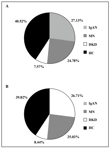
The study workflow is shown in Figure 1. The urinary proteome was treated using an ultrafiltration tube-assisted digestion method that can maintain urinary exosomes and other membrane elements. Tryptic peptides were then analyzed using a high-resolution mass spectrometer. Finally, a total of 610,102 urinary proteomic mass spectra were produced for training and validation of the diagnostic model, including 165,521, 151,159, 46,187, and 247,235 spectra from the IgAN, MN, DKD, and HC groups, respectively. All spectra in each group were randomly divided into a training data set (80%) and a validation data set (20%). As shown in Figure 2, the distribution of the different patient types in the training and validation data sets and the proportions of the kidney disease types were nearly consistent.
Comparison of diagnostic accuracy between XGBoost and other machine learning models
After training, the accuracy of the diagnostic XGBoost model was validated to be 96.03% (95% CI, 95.17%– 96.77%; Table 2). The kappa value was 0.943, and the P value from the McNemar test was 0.00027, which indicate the perfect performance of XGBoost. The RF, SVM, and ANN models were trained in the same way, with accuracy rates of 92.35%, 86.12%, and 87.28%, respectively. The accuracy rates of all the machine learning models tested were relatively high. However, compared with the other models, XGBoost achieved the best performance and was thus applied as our machine learning algorithm (Table 2).
Table 2.
Accuracy of different models in training and validation datasets.
| Model | Accuracy (CI 95%) | |
|---|---|---|
| Training dataset | Validation dataset | |
| Random Forest | 96.36% (95.63%~97.18%) |
92.35% (91.28%~94.23%) |
| Support Vector Machine | 92.67% (89.56%~93.43%) |
86.12% (84.28%~89.71%) |
| Artificial Neural Networks | 95.12% (93.96%~96.71%) |
87.28% (84.27%~90.16%) |
| XGBoost | 99.21% (98.89%~99.48%) |
96.03% (95.17%~96.77%) |
Classification performance of the kidney disease diagnostic XGBoost dodel
To characterize the performance of the diagnostic XGBoost
model for the different types of kidney diseases, we
compared the predictive ability of this model for the three
types of kidney disease and HCs. We chose 20% of the total
data set for the test. Although the number of test errors
was large, the error rate was low.
As shown in Table 3 and Figure 3, the false positivity
rates of the four disease types (IgAN, MN, DKD, and HC)
were 2.76%, 5.73%, 10.19%, and 2.37%, respectively. The
XGBoost model achieved the highest error rate for DKD
and the lowest error rate for IgAN. The accuracy rates for
the three types of kidney disease and HCs were 97.67%,
96.64%, 94.86%, and 97.35%, respectively (Table 4). Although
the accuracy of the diagnosis of each of the four
disease types was extremely high, the diagnostic accuracy
for DKD was the lowest. Comparing four performance items, namely sensitivity, specificity, positive predictive
value, and negative predictive value, we found that the
positive predictive rates for the IgAN and HC groups were
relatively low, as was the sensitivity for both the MN and
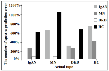
DKD groups. In addition, we specifically analyzed the
misclassification of the four types. As shown in Figure 4,
the IgAN and MN groups were relatively easily misjudged
as the HC group, whereas the DKD and HC groups were
relatively easily misjudged as the IgAN group.
Table 3.
Confusion matrix of XGBoost for diagnosis of chronic kidney diseases.
| Model | Prediction type | Total | False NO. | False rate (1-Sensitiviy) | |||
|---|---|---|---|---|---|---|---|
| IgAN | MN | DKD | HC | ||||
| IgAN | 31700 | 250 | 50 | 600 | 32600 | 900 | 2.76% |
| MN | 650 | 28800 | 50 | 1050 | 30550 | 1750 | 5.73% |
| DKD | 300 | 250 | 9250 | 500 | 10300 | 1050 | 10.19% |
| HC | 750 | 400 | 0 | 47450 | 48600 | 1150 | 2.37% |
| Total | 33400 | 29700 | 9350 | 49600 | 122050 | 4850 | 3.97% |
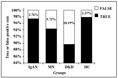
Table 4.
Performance of XGBoost model for diagnosis of chronic kidney diseases.
| Items | IgAN | MN | DKD | HC |
|---|---|---|---|---|
| Sensitivity | 97.24% | 94.27% | 89.81% | 97.63% |
| Specificity | 98.10% | 99.02% | 99.91% | 97.07% |
| Pos-Pred-Value | 94.91% | 96.97% | 98.93% | 95.67% |
| Neg-Pred-Value | 98.98% | 98.11% | 99.01% | 98.41% |
| Balanced accuracy | 97.67% | 96.64% | 94.86% | 97.35% |
Evaluation of the diagnostic XGBoost model for kidney disease
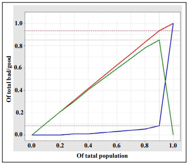
The discrimination ability of the XGBoost diagnostic model for kidney disease was assessed on the basis of the ROC curve and AUC (Figure 5). The AUC of this model was 0.952 (95% CI, 0.9307– 0.9733), demonstrating a strong generalization. In addition, the slope of the gain curve was adequately steep. When the test sample rate was 18.7%, the TPR of the model reached 92.3%, which is high (Figure 6). The KS value of the Lorenz curve was 0.8514, which is much higher than 0.2 (Figure 7). The gain and Lorenz curves also demonstrated the strong robustness of the model.
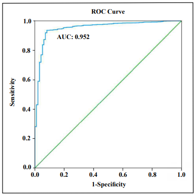
Figure 5. Receiver operating curve (ROC) for estimating the discrimination of XGBoost.
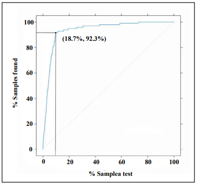
Figure 6. Gain plot for evaluating the overall diagnostic accuracy of the XGBoost model.
Discussion
CKD represents a major public health issue in terms of its
substantial financial burden and consumption of healthcare
resources [1]. In addition, it is a risk factor of hypertension
and cardiovascular diseases, which together
constitute a substantial cause of death in most societies
[22]. Accurate identification and early screening of CKD
in the population have long been important topics. The development
of a noninvasive and accurate early diagnostic
method is needed. The diagnostic ability of a single biomarker
is slightly weak, and renal biopsy is invasive, with
a risk of major bleeding. With the development of mass
spectrometry, urinary proteomes can now be both quantitatively
and qualitatively detected [17]. Our study was focused
on artificial intelligence-assisted noninvasive diagnostic
methods for different types of kidney disease based
on mass spectra information from urinary proteomics.
Previous studies showed that measurement of the
level
of
a single protein marker in the clinical diagnosis of CKD
does not take advantage of the overall value and macro efficiency of proteomics [17]. In addition, the
feasibility
of using a single protein marker in the clinical diagnosis
of CKD requires further research and validation. The use
of several or even dozens of protein panels can improve
the diagnostic accuracy. The existing mass spectrometry
applied in proteomics is used in the identification of differential
proteins and selection of individual proteins for
further differential studies. In fact, the overall data from a
mass spectrometric analysis is not applied. Moreover, the
efficacy of its clinical application requires further evaluation.
By using big data, machine learning can be applied
by integrating all information from a mass spectrometric
analysis. We analyzed all data to take full advantage of
the overall efficiency of proteomic mass spectrometry.
Therefore, for CKD classification, considering the comprehensiveness
of a mass spectrum analysis, as the feature
data of our AI algorithm, we applied a first-order mass
spectrum analysis of the proteomics without further processing.
Artificial intelligence algorithms such as ANNs,
SVMs, DTs, and XGBoost combined with medical or
biological experience have obtained remarkable results
[23, 24]. Through the
training of big data sets, a machine
learning model can predict classifications. Machine learning
outperforms the conventional statistical methods with
its ability to better identify variables, achieve a better
predictive performance and modeling of complex relationships,
and learn from multiple modules of data, and
its robustness against data noise. It has therefore been applied
in the diagnosis of certain diseases such as lung cancer
[25], cardiovascular disease [26], and chronic kidney
disease [27]. Machine and deep learning algorithms can
not only impute missing data in the training sets but also
identify existing characteristics that are otherwise unrecognizable.
Most existing diagnostic machine models for
CKD are based on records and detection indicators that
are currently used in clinical practice [28]. However, the
training data types of these models vary, and the accuracy
of artificial collection is relatively low, with poor clinical
application. To date, no studies have been conducted
on machine learning models for diagnosis based on the
full spectra of CKD urinary proteomics. In addition, of
the many existing machine learning models, XGBoost
achieved an outstanding classification performance without
a high computation time and is a practical approach.
XGBoost is a type of tree-structured model, the basic idea
of which is to design an ensemble approach for several
rule-based binary trees. XGBoost is derived from the most
famous tree ensemble method, called gradient boosting
decision tree. XGBoost has gained popularity by winning
numerous machine learning competitions since its initial
development [18]. Advances in big data and artificial intelligence
have enabled clinicians to process information
more efficiently and make diagnosis and treatment decisions
more accurately [29]. It is unquestionable that big
data and artificial intelligence are transforming medicine
from various perspectives, including precision medicine
and clinical intelligence. On the basis of the big data applied
in urinary proteomic mass spectra, the strategy of using
artificial intelligence and machine learning algorithms has been used to provide a new direction for the
classification
of kidney diseases. To the best of our knowledge, our
study is the first to combine artificial intelligence and urinary
proteomic mass spectra information in the diagnosis
and classification of kidney diseases.
Compared with RF, SVM, and ANNs, the XGBoost model
with mass spectra information for urinary proteomics
showed a perfect performance in the diagnosis of kidney
diseases. This is consistent with the classification ability
of XGBoost models when applied for other clinical
diseases. Therefore, compared with other machine learning
algorithms, the advantages of the XGBoost algorithm
are as follows [30]: First, XGBoost adds a regularization
term to the objective function, which reduces the variance
of the model, simplifying the model while preventing an
overfitting. Second, XGBoost used not only the first derivative
but also the second derivative to make the loss more
accurate. Third, when the training data are sparse, the default
direction of the branch can be specified for a missing
or specified value, which can significantly improve the
efficiency of XGBoost. Fourth, XGBoost supports column
sampling and parallel optimization, thereby reducing the
number of computations and improving efficiency. The
peak value of the urine proteome mass spectrometry data
is presented in the form of a set of numbers in abscissa
and ordinate coordinates, which is used in the construction
of the XGBoost model to maximize such advantages.
In our study, the overall accuracy of the diagnostic XGBoost
model for the four disease groups was 96.03%,
which is basically consistent with the accuracy of renal
biopsy. Therefore, our study highlights the advantages
of using a noninvasive diagnostic method as an artificial
intelligence model in proteomics. In addition, we conducted
a detailed assessment of the modelling accuracy
for each type of kidney disease and the HCs. The specificity
of the diagnostic model for the four disease types
was >95% (97.07%–99.91%); thus, its misdiagnosis rate
is extremely low, and its ability to distinguish each type
of disease shows excellent stability. Although the sensitivity
for the four disease types was approximately 90%
(89.81%–97.63%), the sensitivity for the three types of
kidney disease, excluding the HC group, was lower than
the specificity. Therefore, the missed diagnosis rate of this
model is higher than its misdiagnosis rate, which indicates
that this model may be more suitable for accurate disease
diagnosis than for disease screening. The next steps
of this research will focus on improving the prediction
sensitivity of the model. For all four disease types, the
sensitivity of the model regarding DKD diagnosis was the
worst (89.81%), probably because of the smaller number
of patients with DKD included, smaller mean number of
spectra, or significant differences with the other disease
groups. The low mean number of urinary proteomic mass
spectra is a response to the state of the real disease, which
cannot be avoided. We hope to include more samples in
our future study to reduce the problems caused by data
imbalance. In addition, through analyses of the ROC
curve, gain plot, and Lorenz curve, this study showed that
the model achieved strong robustness and high accuracy.
At present, a few existing XGBoost models for
kidney
disease diagnosis have been constructed using data on the
clinical characteristics and individual laboratory test indicators.
Ogunleye et al. [7] enrolled 250 CKD cases and
150 HCs to train and validate the XGBoost model with 22
clinical features. The accuracy, sensitivity, and specificity
of the XGBoost model were all 100%. Xiao et al. [27]
also constructed a XGBoost model for the prediction of
CKD progression in 551 patients with proteinuria. A total
of 13 blood-derived tests and 5 demographic features
were used as variables to train the model. The accuracy of
this progression model was 0.87. By applying 36 characteristics
of 2,047 Chinese patients from 18 renal centers,
Chen et al. [31] used a XGBoost model for the prediction
of end-stage CKD. The C statistical value of this XGBoost
model was 0.84. As all of these reports were constructed
using clinical information and outcome indicators were
inconsistent, poor comparability with our diagnostic XGBoost
model was achieved. However, the accuracy of our
model is high.
The KDClassifier classified the characteristic differences
of the pathological types of CKD at the level of the integrated
information of mass spectrometry proteomics
in urine. No specific proteins or laboratory indicators of
clinical concern have been identified, such as GFR, urine
protein, or creatinine. This is significantly different from
our normal assumption. The information captured by a
machine learning model is more abundant than that obtained
using comparative analysis of differential proteins.
To explain the specific content of the information captured
by machine learning with human logic requires further
research and discussion.
Overall, the KDClassifier, an XGBoost diagnostic model,
established in this study showed its feasibility and superiority
for clinical application. However, in terms of economics,
the current cost of mass spectrometry analysis of
proteomics is relatively high, and realization of its clinical
application will still take a long time. With further innovations
in science and technology, however, we expect the
cost of mass spectrometric analysis to inevitably decline.
The KDClassifier is not only suitable for the classification
of the three types of kidney disease considered but
also has the potential to be extended to all types of kidney
disease. The diagnostic advantages of this model will be
fully demonstrated.
Our study also has certain limitations. First, the cohort
used was not from a prospective trial, and selective bias
was inevitable. Second, only three common types of kidney
disease were included. Whether this learning machine
diagnostic method is suitable for other types of kidney
disease needs further research and validation using a larger
sample size. Third, owing to the relatively small sample
size, we did not include more clinical parameters for an
artificial intelligence-assisted analysis. Including more
clinical data will further improve the diagnostic power of
our model. Fourth, this study only compared four mainstream
machine learning methods with certain limitations.
Fifth, only the mass spectra of urinary proteomic information
were used, and the clinical information of the patients was omitted. If both types of information are
combined,
patients can be better diagnosed. We expect to develop
more suitable artificial intelligence algorithms for a noninvasive
and accurate diagnosis of kidney diseases.
Conclusion
In conclusion, the KDClassifier, a machine learning classification model that applies information on mass spectra from urinary proteomics, showed high accuracy in the diagnosis of different types of CKD. This study provides new insights into the application of artificial intelligence in the accurate and noninvasive diagnosis of kidney diseases. In addition, the KDClassifier provides a potential tool for the classification of all types of kidney disease.
Declarations
Funding
This work was funded by grants from the National Natural Science Foundation of China (grant no. 31901038), the China Postdoctoral Science Foundation (2019M653438), the Post-Doctoral Research Foundation of West China Hospital of Sichuan University (2018HXBH062/2018HXBH074).
Conflicts of interest
The authors declare no conflict of interest.
Availability of data and material
The mass spectra data on the urinary proteomics were deposited into the ProteomeXchange Consortium through the PRIDE partner repository using the dataset identifier PXD018996.
Code availability
The codes that support the findings of this study are available on request from the corresponding author. The codes are not publicly available due to privacy or ethical restrictions.
Statement
We confirm that all methods were carried out in accordance with relevant guidelines and regulations in the manuscript.
Authors’ contributions
G.L., H.Y., J.C., J.Z. and F.L.
directed and designed research;
Y.Z. Y.M.and W.Z. directed and performed analyses of
mass spectrometry data;
W. Z., X.L. and Y.M. adapted algorithms and software for
data analysis;
C.W. and L.Z. coordinated acquisition, distribution and
quality evaluation of samples;
W.Z. and Y.Z. wrote the manuscript.
References
1. Coresh J. Update on the Burden of CKD. Journal of the American Society of Nephrology, 2017, 28(4): 1020- 1022.
2. Xie Y, Bowe B, Mokdad AH, et al. Analysis of the Global Burden of Disease study highlights the global, regional, and national trends of chronic kidney disease epidemiology from 1990 to 2016. Kidney International, 2018, 94(3): 567-581.
3. Glassock RJ, Warnock DG, Delanaye P. The global burden of chronic kidney disease: estimates, variability and pitfalls. Nature Reviews Nephrology, 2017, 13(2): 104-114.
4. Okparavero A, Foster MC, Tighiouart H, et al. Prevalence and complications of chronic kidney disease in a representative elderly population in Iceland. Nephrology Dialysis Transplantation, 2016, 31(3): 439-447.
5. Marcussen N, Olsen S, Larsen S, et al. Reproducibility of the WHO classification of glomerulonephritis. Clinical Nephrology, 1995, 44(4): 220-224.
6. Sethi S, Haas M, Markowitz GS, et al. Mayo Clinic/Renal Pathology Society Consensus Report on Pathologic Classification, Diagnosis, and Reporting of GN. Journal of the American Society of Nephrology, 2016, 27(5): 1278- 1287.
7. Fogo AB. Morphology expands understanding of lesions. Kidney International, 2020, 97(4): 627-360.
8. Lemley KV. Machine Learning Comes to Nephrology. Journal of the American Society of Nephrology, 2019, 30(10): 1780-1781.
9. Hermsen M, de Bel T, den Boer M, et al. Deep Learning- Based Histopathologic Assessment of Kidney Tissue. Journal of the American Society of Nephrology, 2019, 30(10): 1968-1979.
10. Sekulic M, Crary GS. Kidney Biopsy Yield: An Examination of Influencing Factors. American Journal Of Surgical Pathology, 2017, 41(7): 961-972.
11. Ito S. Aneurysmal dilatation associated with arteriovenous fistula in a transplanted kidney after renal biopsies. Pediatric Transplantation, 2014, 18(7): E216-E219.
12. Lin RC. Lipidomics: new insight into kidney disease. Advances in Clinical Chemistry, 2015, 68: 153-175.
13. Zhao YY. Metabolomics in chronic kidney disease. Clinica Chimica Acta, 2013, 422: 59-69.
14. Wu J, Chen YD, Gu W. Urinary proteomics as a novel tool for biomarker discovery in kidney diseases. Journal of Zhejiang University-Science B, 2010, 11(4): 227-237.
15. Beck LH, Bonegio RGB, Lambeau G, et al. M-Type Phospholipase A(sub 2) Receptor as Target Antigen in Idiopathic Membranous Nephropathy. New England Journal of Medicine, 2009, 361(1): 11-21.
16. Scheubert K, Hufsky F, Petras D, et al. Significance estimation for large scale metabolomics annotations by spectral matching. Nature Communications, 2017, 8(1): 1-10.
17. Mischak H, Delles C, Vlahou A, et al. Proteomic biomarkers in kidney disease: issues in development and implementation. Nature Reviews Nephrology, 2015, 11(4): 221-232.
18. Chen TQ, Guestrin C. XGBoost: A Scalable Tree Boosting System. Kdd’16: Proceedings of the 22nd Acm Sigkdd International Conference on Knowledge Discovery and Data Mining. 2016: 785-794.
19. Xie N, Chu CL, Tian XY, et al. An Endogenous Project Performance Evaluation Approach Based on Random Forests and IN-PROMETHEE II Methods. Mathematical Problems in Engineering, 2014.
20. Sang YS, Zhang HX, Zuo L. Least Squares Support Vector Machine Classifiers Using PCNNs. 2008 Ieee Conference on Cybernetics and Intelligent Systems, Vols 1 and 2, 2008: 828-833.
21. Goodacre R, Kell DB. Correction of mass spectral drift using artificial neural networks. Analytical Chemistry, 1996, 68(2): 271-280.
22. Ene-Iordache B, Perico N, Bikbov B, et al. Chronic kidney disease and cardiovascular risk in six regions of the world (ISN-KDDC): a cross-sectional study. Lancet Global Health. 2016, 4(5): e307-319.
23. Delahunt CB, Mehanian C, Hu LM, et al. Automated Microscopy and Machine Learning for Expert-Level Malaria Field Diagnosis. Proceedings of the Fifth Ieee Global Humanitarian Technology Conference Ghtc 2015, 2015: 393-399.
24. Mandal S. A Survey of Adaptive Fuzzy Controllers: Nonlinearities and Classifications. IEEE Transactions on Fuzzy Systems, 2015, 24(5): 1095-1107.
25. Baxi V, Beck A, Pandya D, et al. Artificial intelligencepowered retrospective analysis of PD-L1 expression in nivolumab trials of advanced non-small cell lung cancer. Journal for Immunotherapy of Cancer, 2019, 7.
26. Tsipouras MG, Voglis C, Fotiadis DI. A framework for fuzzy expert system creation - Application to cardiovascular diseases. Ieee Transactions on Biomedical Engineering, 2007, 54(11): 2089-2105.
27. Xiao J, Ding RF, Xu XL, et al. Comparison and development of machine learning tools in the prediction of chronic kidney disease progression. Journal of Translational Medicine, 2019, 17(1): 1-13.
28. Ogunleye AA, Qing-Guo W. XGBoost Model for Chronic Kidney Disease Diagnosis. IEEE-ACM Transactions on Computational Biology and Bioinformatics, 2019, 17(6): 2131-2140.
29. Yang C, Kong GL, Wang LW, et al. Big data in nephrology: Are we ready for the change? Nephrology, 2019, 24(11): 1097-1102.
30. Li CB, Zheng XS, Yang ZK, et al. Predicting Short-Term Electricity Demand by Combining the Advantages of ARMA and XGBoost in Fog Computing Environment. Wireless Communications & Mobile Computing, 2018.
31. Chen TY, Li X, Li YX, et al. Prediction and Risk Stratification of Kidney Outcomes in Iga Nephropathy. American Journal of Kidney Diseases, 2019, 74(3): 300-309.